Splines to piecewise functions

by Sergio Rossell - 27 Jan 2021

Tags: #Stan #Bayes #ODEs

Building piecewise functions from splines.

In this notebook I show how to build piecewse functions from splines using Scipy. If you stay within Python there may be no need for building a piecewise function. My motivation raised from the desire to use splines fitted to data as inputs for modeling in Stan.

I took ideas from two stackoverflow posts. The first shows how to build piecewise functions from Scipy's CubicSpline. The second shows how to build piecewise functions from Scipy's UnivariateSpline.

As an example, I use the example shown in Scipy's UnivariateSpline, with a offset to avoid negative number. Then I show how to use build, from a UnivariateSpline instance, a piecewise function that works in Stan.

Piecewise representation of a cubic spline with four knots

$$y(x) = \begin{cases} y_0\cdot (x-x_0) + b_0 \cdot (x-x_0) + c_0 \cdot (x-x_0)^2 + d_0\cdot (x-x_0)^3 & \in [x_0, x_1) \\ y_1\cdot (x-x_1) + b_1 \cdot (x-x_1) + c_1 \cdot (x-x_1)^2 + d_1\cdot (x-x_1)^3 & \in [x_1, x_2) \\ y_2\cdot (x-x_2) + b_2 \cdot (x-x_2) + c_2 \cdot (x-x_2)^2 + d_2\cdot (x-x_2)^3 & \in [x_2, x_3] \end{cases}$$

How to get this representation from Scipy's UnivariateSpline:

Create data.

import numpy as np

data_x = np.linspace(-3, 3, 50)
data_y = 0.2 + np.exp(-data_x**2) + 0.1 * np.random.randn(50)  # NOTE I added the 0.2 offset

Fit a spline and extract the coeffients

from scipy.interpolate import PPoly, UnivariateSpline

smoothing_factor = 0.8  # Selected to obatain a reasonable fit with a low number of knots
k = 3  # The order of the spline, i.e. cubic.
n = 20  # number of points per segment when plotting the resulting spline

spl = UnivariateSpline(data_x, data_y, s=smoothing_factor, k=3)
# getting a piecewise polynomial from the spline
p_spl = PPoly.from_spline(spl._eval_args)

The spline object p_spl includes the location of the knots, which define the segments, and the coefficients of the piecewise representation of the spline.

p_x = p_spl.x[k:-k]
p_c = p_spl.c[:, k:-k]

#### A pretty table of the coefficients using pandas
import pandas as pd
pd.DataFrame(p_c, index=list("ybcd"), columns=[f"segment_{i}" for i in range(p_c.shape[1])])

coeff	segment_0	segment_1	segment_2
y	-0.168	0.233	-0.0928
b	0.920	-0.626	0.400
c	-1.022	-0.120	-0.452
d	0.415	1.081	0.290

Depending on you application you may wish to use a vecotized function (which I call here piecewise_segment) or a point by point function (piecewise_point)

piecewise_segment = lambda x, x0, c_col_vec: c_col_vec @ ((x - x0)[np.newaxis, :] ** np.arange(k + 1)[::-1, np.newaxis])
piecewise_point = lambda x, x0, c_col_vec: c_col_vec @ ((x - x0) ** np.arange(k + 1)[::-1])

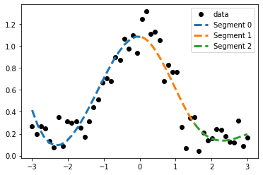
An illustration of the segements in the piecewise function.

The start and end of the segments is given by the knots of the spline regression.

fig, ax = plt.subplots()
ax.plot(data_x, data_y, 'ko', label="data");
for i in range(p_x.shape[0] - 1):
    segment_x = np.linspace(p_x[i], p_x[i + 1], n)
    segment_y = piecewise_segment(segment_x, p_x[i], p_c[:, i])# .dot(exp_x)  # s.c[:, 1] @ exp_x
    ax.plot(segment_x, segment_y, label='Segment {}'.format(i), ls='--', lw=3)
ax.legend();

piecewisespline

Python example of a piecewise function

Which could be used, for instance, as an input for an ordinary differential equation solver.

triplets = zip(range(p_x.shape[0] - 1), p_x[:-1], np.roll(p_x, -1)[:-1])
conditions = ""
functions = ""
fl = []
body = ""
for i, lb, ub in triplets:
    if i == 0:
        body += f"    if (x >= {lb}) & (x <= {ub}):\n"
        body += f"        y = piecewise_point(x, {lb}, p_c[:, {i}])\n"
    else:
        body += f"    elif (x > {lb}) & (x <= {ub}):\n"
        body += f"        y = piecewise_point(x, {lb}, p_c[:, {i}])\n"

        pw_spline_str = f"""
def pw_spline(x):
{body}
    else:
       y = None
    return y
"""
print(pw_spline_str)

def pw_spline(x):
    if (x >= -3.0) & (x <= 0.06122448979591821):
        y = piecewise_point(x, -3.0, p_c[:, 0])
    elif (x > 0.06122448979591821) & (x <= 1.5306122448979593):
        y = piecewise_point(x, 0.06122448979591821, p_c[:, 1])
    elif (x > 1.5306122448979593) & (x <= 3.0):
        y = piecewise_point(x, 1.5306122448979593, p_c[:, 2])

    else:
       y = None
    return y

Python code to write and run a stan model

"""
Noiseless simulation of a system of ordinary equations driven by a spline input
using Stan.

The system of odes represents a simple linear chain of enzyme catalyzed
reactions:

    -> x1 -> x2

The rate of the first reaction (arrow) is simulated as a spline function, the
rate of the second reaction is catalyzed by an enzyme described with
irreversible Michaelis-Menten kinetics.
"""
from scipy.interpolate import PPoly, UnivariateSpline

import matplotlib.pyplot as plt
import numpy as np
import pandas as pd
import pystan

np.random.seed(1235)
###############################################################################
# INPUTS

stan_str0 = """
functions {{
    real[] bwp (
        real x,
        int k
    )
    {{
    real res[(k + 1)];
    for (p in 1:(k + 1)) {{
        res[p] = pow(x, ((k + 1) - p));
        }}
    return res;
    }}

    real piecewise_point (
        real x,
        real x0,
        int i,
        int k,
        int c_dim1,  // num rows c matrix
        int c_dim0,  // num cols c matrix
        real[] c_flat  // flattened C matrix
    )
    {{
        row_vector[4] x2pow;
        vector[4] c_col;
        real y;
        x2pow = to_row_vector(bwp((x-x0), k));
        c_col = col(to_matrix(c_flat, c_dim0, c_dim1), i);
        y = dot_product(x2pow, c_col);
        return y;
    }}

{pw_spline}

    real f_mm (
        real[] y
    )
    {{
        real v_mm;
        v_mm = (y[1]/1) / (1 + (y[1]/1));
        return v_mm;
    }}

    real[] myodes(
        real t,
        real[] y,
        real[] p,
        real[] x_r,
        int [] x_i
        )
        {{
            real dydt[2];
            dydt[1] = pw_spline(t, x_r, x_i[1], x_i[2], x_i[3]) - f_mm(y);
            dydt[2] = f_mm(y);
            return dydt;
        }}
}}

data {{
    int<lower=1> k;  // order plus 1
    int<lower=1> T;
    int<lower=1> c_dim0;
    int<lower=1> c_dim1;
    int<lower=1> c_flat_dim0;
    real c_flat[c_flat_dim0];
    real t0;
    real t_sim[T];
    real<lower=0> y0[2]; // init
    }}

transformed data {{
    real x_r[0];
    int x_i[3];
    x_i[1] = k;
    x_i[2] = c_dim0;
    x_i[3] = c_dim1;
}}

parameters {{
    vector<lower=0>[2] sigma;
    real<lower=0> p[0];
}}

transformed parameters {{
    real x0;
    real y_hat[T, 2];
    y_hat = integrate_ode_rk45(myodes, y0, t0, t_sim, p, c_flat, x_i);
}}

model {{
}}

generated quantities {{
}}
"""

# Synthetic data to fit a spline to (from UnivariateSpline documenation)
# https://docs.scipy.org/doc/scipy/reference/generated/scipy.interpolate.UnivariateSpline.html#scipy.interpolate.UnivariateSpline
data_x = np.linspace(-3, 3, 50)
# NOTE. I added 0.2 to data_y to avoid negative numbers
data_y = 0.2 + np.exp(-(data_x ** 2)) + 0.1 * np.random.randn(50)

# Smoothing factor for UnivariateSpline. Tuned to give four knots
smoothing_factor = 0.8

# Time vector for simulation
t_sim = np.arange(-2.9, 3.1, 0.1)

###############################################################################
# STATEMENTS

# fit a spline
spl = UnivariateSpline(data_x, data_y, s=smoothing_factor)

# getting a piecewise polynomial from the spline
p_spl = PPoly.from_spline(spl._eval_args)

p_x = p_spl.x[3:-3]
p_c = p_spl.c[:, 3:-3]

# Creating piecewise function from spline
triplet = zip(range(1, p_x.shape[0]), p_x[:-1], np.roll(p_x, -1)[:-1])
body = ""
for i, lb, ub in triplet:
    if i == 1:
        body += f"        if ((x >= {lb}) && (x <= {ub}))\n"
        body += (
            f"            y = piecewise_point(x, {lb}, {i}, k, c_dim0, c_dim1, c);\n"
        )
    elif i == (p_x.shape[0] - 1):
        body += f"        else  // ((x > {lb}) && (x <= {ub}))\n"
        body += f"            y = piecewise_point(x, {lb}, {i}, k, c_dim0, c_dim1, c);"
    else:
        body += f"        else if ((x > {lb}) && (x <= {ub}))\n"
        body += (
            f"            y = piecewise_point(x, {lb}, {i}, k, c_dim0, c_dim1, c);\n"
        )


pw_spline_str = f"""
    real pw_spline (
        real x,
        real[] c,
        int k,
        int c_dim1,  // num rows c matrix
        int c_dim0  // num cols c matrix
    )
    {{
    real y;
{body}
    return y;
    }}
"""

stan_str = stan_str0.format(pw_spline=pw_spline_str)

# Dictionary to pass to the stan model
datadict = {}
datadict["k"] = 3  # Degree of the spline to fit (i.e. cubic)
datadict["c_dim0"] = p_c.shape[0]
datadict["c_dim1"] = p_c.shape[1]
datadict["c_flat"] = p_c.flatten(order="F")
datadict["c_flat_dim0"] = p_c.flatten(order="F").shape[0]
datadict["t0"] = -3.0
datadict["t_sim"] = t_sim
datadict["T"] = len(t_sim)
datadict["y0"] = [0, 0]

# compile StanModel
sm = pystan.StanModel(model_code=stan_str)

fit = sm.sampling(
    data=datadict, iter=1, chains=1, n_jobs=1, algorithm="Fixed_param", seed=42
)

summary = fit.summary()
df_summary = pd.DataFrame(
    summary["summary"],
    columns=summary["summary_colnames"],
    index=summary["summary_rownames"],
)

fit_dict = fit.extract()
fit_df = pd.DataFrame(fit_dict["y_hat"][0], index=t_sim, columns=["x1", "x2"])

fit_df.plot(subplots=True)
plt.show()